VULNADO! Lots of Bugs, Not So Many Bites / Gunnar Leffler

Vulnado! CVEs Since 1999.

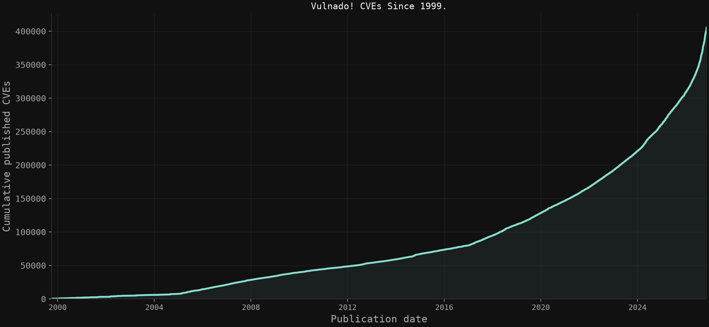
Hide yo stacks, hide yo racks. They’re assigning CVEs to everything out here.

I'm sure you've seen these big, scary, exponential-looking CVE graphs bandied about in infosec circles online. Add LLMs finding long-hidden cracks in our software infrastructure, and the story gets louder: discoveries arriving at a furious rate, decades-old bugs surfacing overnight. I even remember seeing a claim that “3% of all compromises in computing history happened in the last week.” I can’t find the source now, but the line stuck with me. Can we believe it? What would that number even measure? I decided to dig into the numbers and see what they actually mean: what gets published, who gets credited, and how much of it shows up in evidence of exploitation.

Breaking Down the Growth

From SQLite to insight with tslite

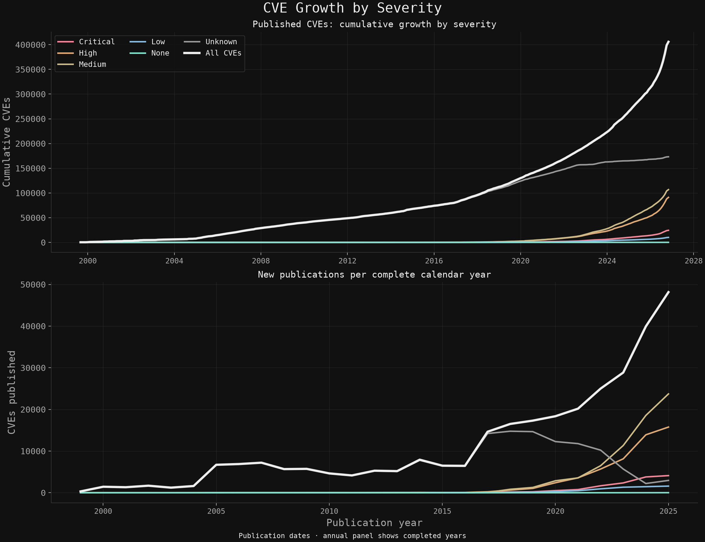
From indexed CVE records to a cumulative publication curve. This compact example counts all severities together; the chart above also splits them by severity.

import sqlite3
import matplotlib.pyplot as plt
# Lightweight time-series tools, ready to work with your query results.
from tslite import timeseries

# Run from the cve_analysis directory after building the index.
with sqlite3.connect("file:analysis.sqlite3?mode=ro", uri=True) as db:
    rows = db.execute("""
        SELECT substr(published_at, 1, 7) || '-01', count(*)
        FROM cves
        WHERE state = 'PUBLISHED' AND published_at IS NOT NULL
        GROUP BY 1 ORDER BY 1
    """).fetchall()

# tslite auto-parses dates: SQLite rows go straight into a series.
monthly = timeseries(rows)
# Accumulate and send to Matplotlib in one easy-to-read line.
plt.plot(*monthly.runningTotal().toPlot(), label="All CVEs")
plt.legend()

To conduct this analysis I downloaded data (see references) into SQLite and used my personal time-series library, tslite.

The cumulative CVE curve is getting steep, but the annual numbers tell us what’s driving it. Publications went from about 20,000 in 2021 to 48,000 in 2025, the last complete year on the chart. Of those 48,000, roughly 24,000 were rated Medium and another 16,000 were rated High. Critical CVEs rose too, but they accounted for only about 4,000. The growth is real. It’s mostly in the middle.

There’s another wrinkle. A lot of older CVEs in this dataset have no severity rating, and that bucket has shrunk in recent years. So I wouldn’t read the severity lines as a clean measure of how much more dangerous software has gotten. They reflect what got published and what got scored.

That’s the distinction I want to carry into the next chart. We’re publishing a lot more vulnerabilities, including a lot more rated High. How many more are attackers actually using?

Shameless plug for tslite:

I've been maintaining it on and off since 2009, mostly to make working with timestamped measurements straightforward. It's a single Python module that lets you slice and dice, manipulate, concatenate and visualize time-series data. It natively works with SQLite storage.

The idea is composability: so you can use small operations to build a more interesting calculation just by chaining them. Query some counts, pass the rows into timeseries(), and let it parse the dates and sort the observations. Add related series, accumulate the totals, smooth a noisy signal, or select a time range. Most transformations return a new series, leaving the original observations alone; toPlot() hands timestamps and values straight to Matplotlib.

The expandable examples below show the SQLite-to-plot workflow.

CVE Attribution

Example Code

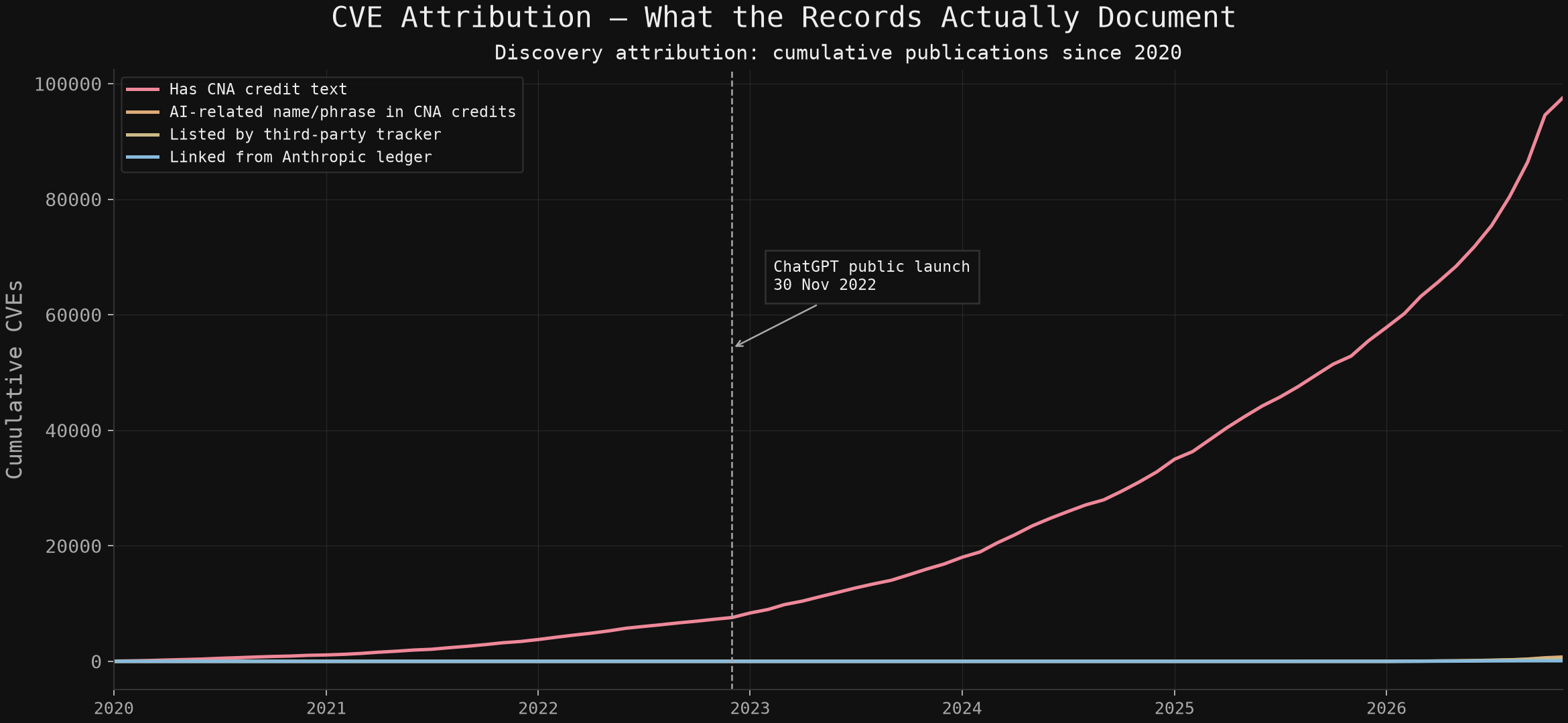
Select ledger-linked CVEs, then accumulate their monthly publications. EXISTS keeps each CVE counted once.

import sqlite3
import matplotlib.pyplot as plt
# Lightweight time-series tools, ready to work with your query results.
from tslite import timeseries

# Run from the cve_analysis directory after building the index.
with sqlite3.connect("file:analysis.sqlite3?mode=ro", uri=True) as db:
    rows = db.execute("""
        SELECT substr(c.published_at, 1, 7) || '-01', count(*)
        FROM cves AS c
        WHERE c.state = 'PUBLISHED' AND c.published_at IS NOT NULL
          AND EXISTS (SELECT 1 FROM finding_cves AS f
                      WHERE f.cve_id = c.cve_id)
        GROUP BY 1 ORDER BY 1
    """).fetchall()

# tslite auto-parses the dates and keeps observations in time order.
monthly = timeseries(rows)
# Running totals to plot-ready data: just chain the operations.
plt.plot(*monthly.runningTotal().toPlot(), label="Ledger-linked CVEs")
plt.legend()

Who Gets the Credit?

In April 2026, Anthropic withheld Claude Mythos Preview from public release because of its reported ability to find and exploit software vulnerabilities. It claims the model found thousands of previously unknown flaws across major operating systems and browsers, and that Anthropic engineers without formal security training were able to get working exploits overnight.

Rather than release the model publicly to us plebes, Anthropic launched Project Glasswing, a defensive initiative backed by up to $100 million in model usage credits. The stated goal was to give organizations including Apple, Google, Microsoft, AWS, and NVIDIA a head start on finding and fixing vulnerabilities before similarly capable models became widely available.

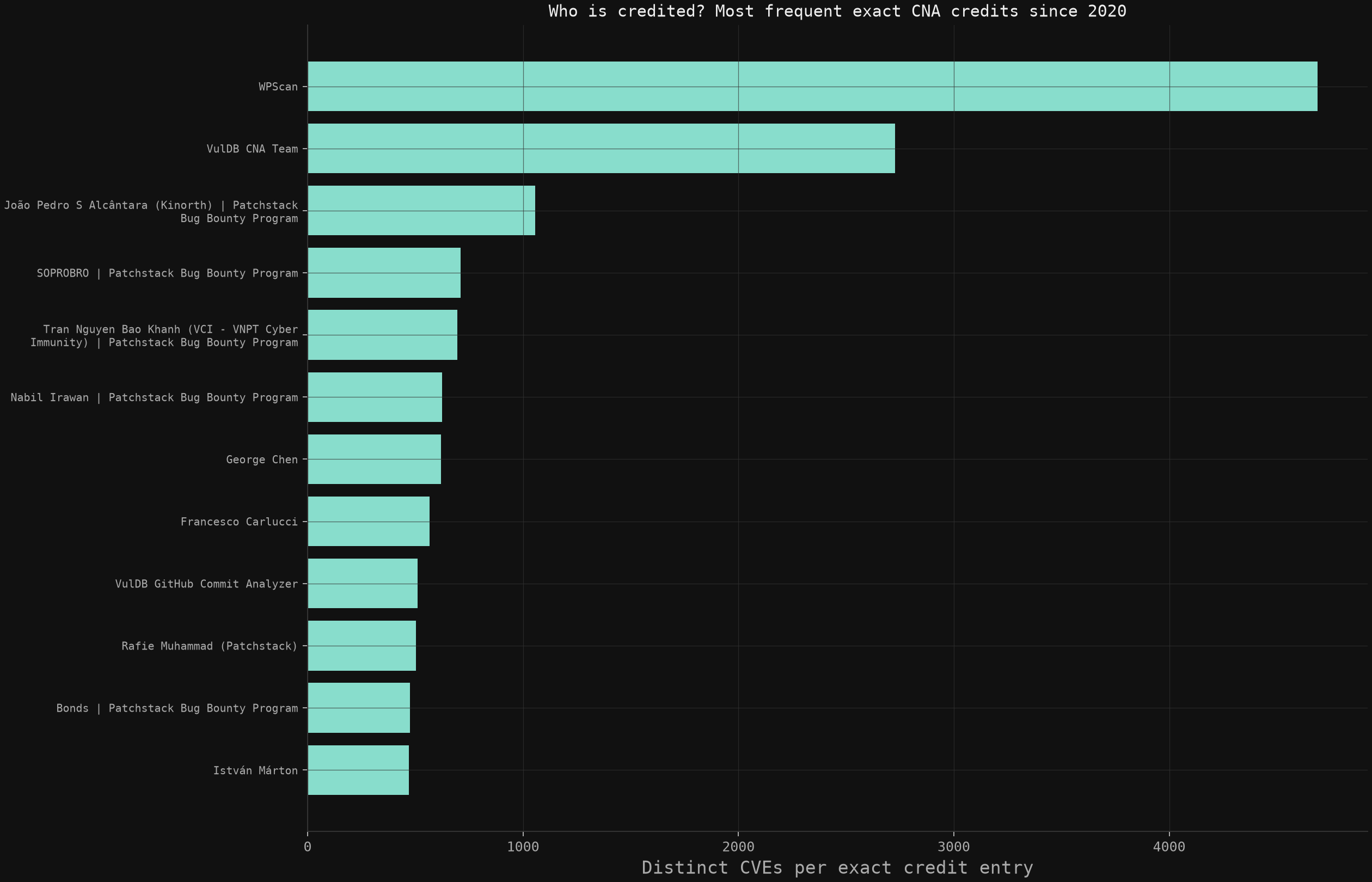
As you can see in the attribution plots above, the most prolific bug finders are Independent researchers, ostensibly accelerating their workflow using LLMs. The Frontier labs are that little sliver on the bottom right

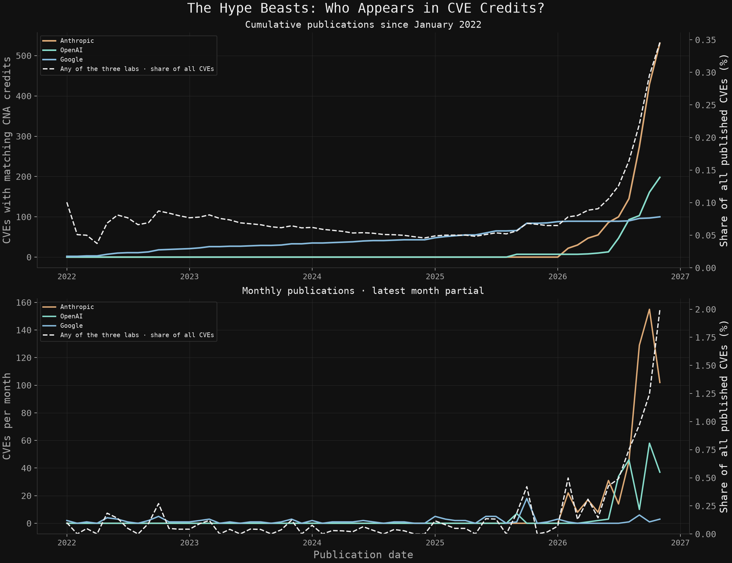
The Hype Beasts

Example Code

Combined lab credits and their share of all publications, with separate count and percentage axes. Uses the same name-matching rules as the full chart; CVEs shared by labs count once.

import re
import sqlite3
import matplotlib.pyplot as plt
from plot_hype import PATTERNS
# Small, composable tools for counts, percentages and plotting.
from tslite import timeseries

pattern = re.compile('|'.join(PATTERNS.values()), re.I)
with sqlite3.connect("file:analysis.sqlite3?mode=ro", uri=True) as db:
    db.create_function("lab_credit", 1, lambda text: bool(pattern.search(text or '')))
    rows = db.execute("""
        WITH labs AS (
            SELECT DISTINCT cve_id FROM credits WHERE lab_credit(value)
        )
        SELECT substr(c.published_at, 1, 7) || '-01', count(*), count(l.cve_id)
        FROM cves AS c LEFT JOIN labs AS l ON l.cve_id = c.cve_id
        WHERE c.state = 'PUBLISHED' AND c.published_at >= '2022-01-01'
        GROUP BY 1 ORDER BY 1
    """).fetchall()

# tslite auto-parses SQL dates into an aligned publication series.
published = timeseries([(t, total) for t, total, labs in rows])
# One observation per month, with shared lab credits deduplicated.
credited = timeseries([(t, labs) for t, total, labs in rows])
# Aligned percentages are a single composable operation.
share = credited.percent(published)
fig, left = plt.subplots()
# toPlot() hands the count series straight to Matplotlib.
left.plot(*credited.toPlot(), color='#88ddcc', label='Three labs combined')
left.set_ylabel('Credited CVEs per month')
right = left.twinx()
# The same easy handoff works on a second percentage axis.
right.plot(*share.toPlot(), color='#eeeeee', linestyle='--', label='Share of all CVEs')
right.set_ylabel('Share of all published CVEs (%)')
left.legend(loc='upper left')
right.legend(loc='upper right')

Let’s take a closer look at the Hype Beasts (aka Frontier Labs) and their little slice of the pie.

Google’s CVE credits have accumulated at a roughly steady pace since 2022. In 2026, Anthropic and OpenAI started showing up much more often, with Anthropic driving most of the late-year spike. Even then, the three labs combined were credited on about 2% of published CVEs in the latest, still-incomplete month.

So what did those hundreds of millions in announced commitments actually get us? The chart tells us who got credit, but how many of those bugs mattered to attackers, how many fixes made it into production, or how much harder any of us are to break into?

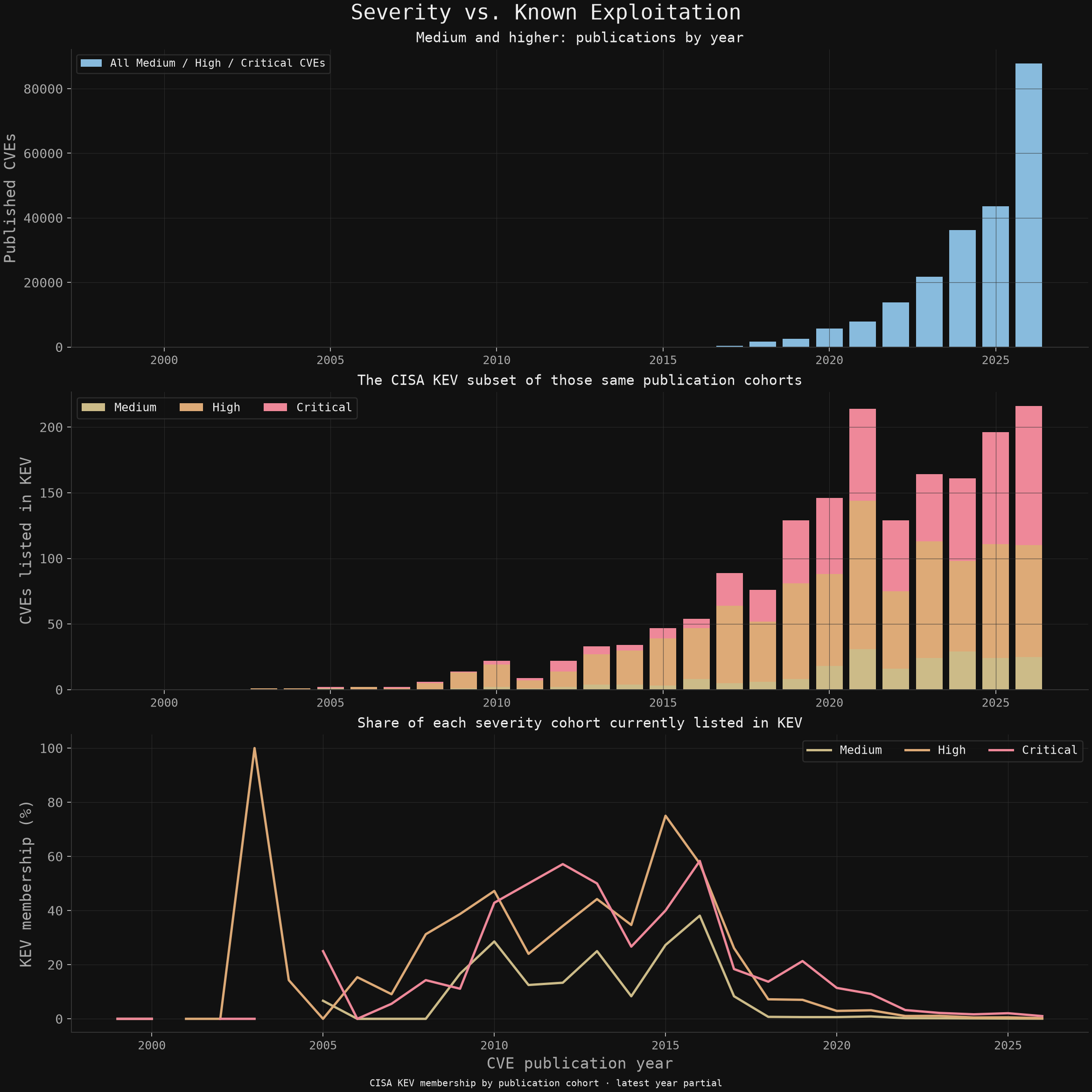
Severity vs. Known Exploitation

Example Code

One query produces aligned publication and KEV counts. tslite turns them into percentages. For brevity this example includes all severities; the chart above uses separate severity cohorts.

import sqlite3
import matplotlib.pyplot as plt
# Lightweight time-series tools, ready to work with your query results.
from tslite import timeseries

# Run from the cve_analysis directory after building the index.
with sqlite3.connect("file:analysis.sqlite3?mode=ro", uri=True) as db:
    rows = db.execute("""
        SELECT substr(c.published_at, 1, 4) || '-01-01',
               count(*), count(k.cve_id)
        FROM cves AS c
        LEFT JOIN kev_entries AS k ON k.cve_id = c.cve_id
        WHERE c.state = 'PUBLISHED' AND c.published_at IS NOT NULL
        GROUP BY 1 ORDER BY 1
    """).fetchall()

# Pick the publication counts; tslite auto-parses their date strings.
published = timeseries([(t, n) for t, n, k in rows])
# Same dates, different measurement—ready for aligned comparisons.
kev = timeseries([(t, k) for t, n, k in rows])
# Calculate aligned percentages and send them straight to Matplotlib.
plt.plot(*kev.percent(published).toPlot(), label="Currently in CISA KEV (%)")
plt.legend()

The Vulnpocalypse has a denominator problem. We’re publishing far more CVEs, but a shrinking share show up in either CISA’s Known Exploited Vulnerabilities catalog or Shadowserver’s honeypot data. That trend was already underway before LLMs went mainstream. If each new batch of CVEs were as useful to attackers as the last, you’d expect the number they’re seen targeting to grow roughly in step with disclosures. It hasn’t.

The overwhelming majority of CVEs just aren’t that useful to attackers. That doesn’t make them fake bugs. It means attackers have a job to do, and a random flaw in a random product usually doesn’t help them do it. Even a Critical rating doesn’t tell you whether the product is widely deployed, whether the vulnerable configuration is reachable, or whether exploiting it gets an attacker anything they can’t get more reliably another way.

AI can make bug hunting faster. It can even make some exploits cheaper to develop. Neither makes the average bug more worth exploiting. The disclosure flood is real, and so is the extra work it creates for defenders. But a bigger triage queue isn’t a cyber apocalypse. So far, it looks like much ado about not much.

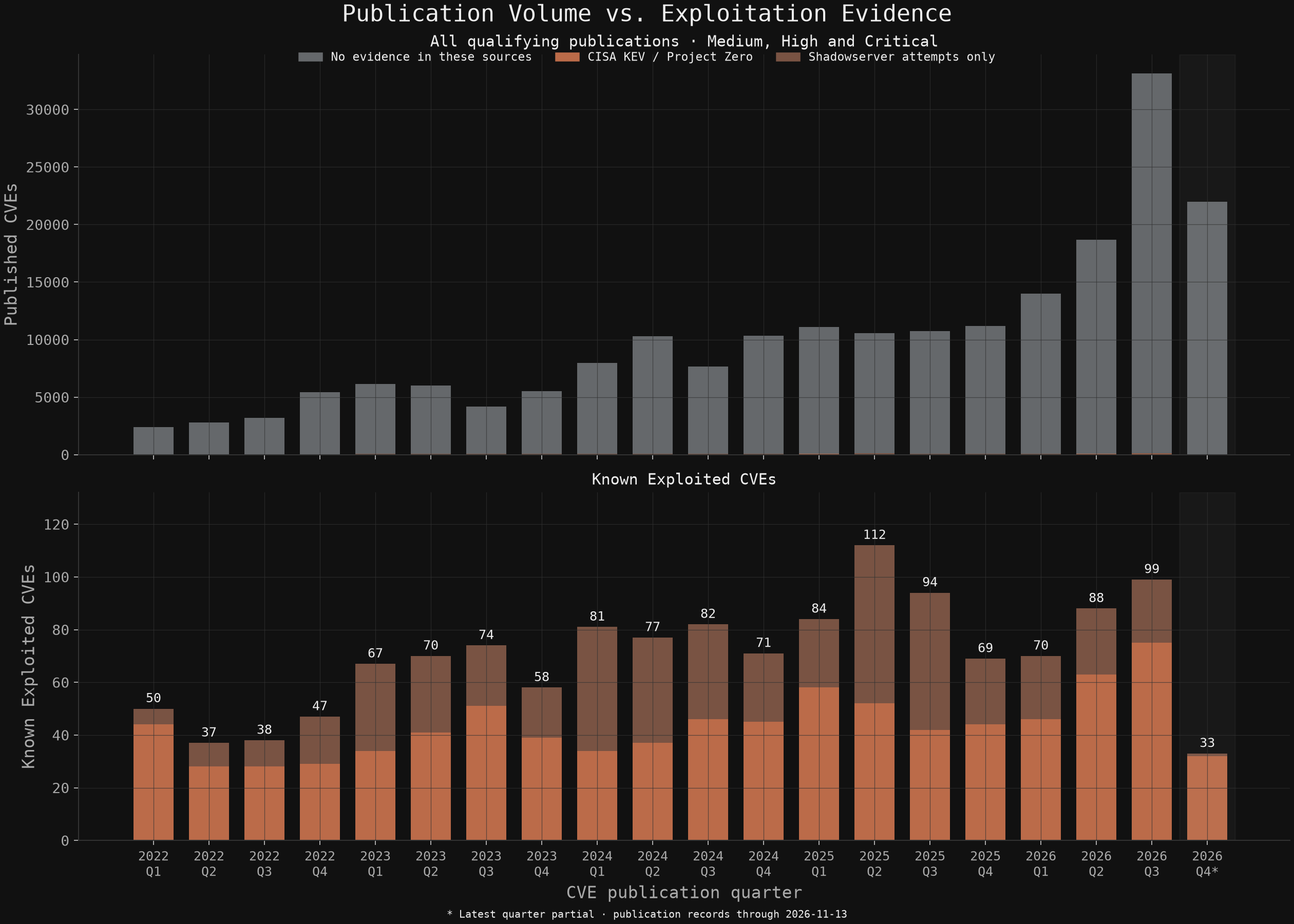
Publication Volume vs. Exploitation Evidence

Example Code

A compact all-severity example: SQL counts by publication quarter, tslite holds the resulting observations, and Matplotlib draws the bars. The full chart additionally applies severity and evidence classifications.

import sqlite3
import matplotlib.pyplot as plt
# Lightweight time-series tools, ready to work with your query results.
from tslite import timeseries

# Run from the cve_analysis directory after building the index.
with sqlite3.connect("file:analysis.sqlite3?mode=ro", uri=True) as db:
    rows = db.execute("""
        SELECT printf('%s-%02d-01', substr(published_at, 1, 4),
                      1 + 3 * ((cast(substr(published_at, 6, 2) AS int)-1)/3)),
               count(*)
        FROM cves
        WHERE state = 'PUBLISHED' AND published_at IS NOT NULL
        GROUP BY 1 ORDER BY 1
    """).fetchall()

# tslite auto-parses dates—even quarterly SQL results drop straight in.
quarterly = timeseries(rows)
# Straight from series to bars—toPlot() makes the handoff effortless.
plt.bar(*quarterly.toPlot(), width=65, label="Publications per quarter")
plt.legend()

These plots show show roughly twice as many medium-or-higher CVEs, about 10% more KEV entries, and no comparable surge in honeypot sightings. Essentially, CVE's can be real bugs and still have little value to an attacker. If AI were turning a big share of the new disclosures into useful exploits, I’d expect some of that to show up in KEV or Shadowserver.

The distinction that the hype glosses over is that AI can make vulnerability analysis and exploit development cheaper without making the underlying target more valuable. It doesn’t put the affected product on the internet, remove a login prerequisite, or give an attacker a reason to switch from a reliable exploit they already have. The case for guardrails can rest on a small number of high-impact bugs. That’s different from claiming the whole disclosure spike is a wave of new opportunities for skids or even seasoned attackers.

A few bugs can ruin your weekend. To be clear there will come a day when nasty, point and shoot exploits will be found. That doesn’t make the whole slop pile an emergency.

Vulnado! CVEs Since 1999.

Breaking Down the Growth

Shameless plug for tslite:

CVE Attribution

Who Gets the Credit?

The Hype Beasts

Severity vs. Known Exploitation

Publication Volume vs. Exploitation Evidence

References